
Put on your favorite space hat and get ready to explore the nascent frontier of quantum computation! While quantum computation still smacks of being futuristic science fiction magic, it's nevertheless beginning to enter into mainstream programming in the here and now.
IBM has unveiled its cloud quantum computer for public use, Microsoft has revealed the Q# quantum programming language, and D-Wave Systems partnered with NASA to release the D-Wave-2.
Being the good futurologists that we are, we'll spend today's article exploring Quantum Computation libraries in Python and JavaScript in order to gain some increased familiarity with this powerful new technology.
Classical Computation
Classical bits are represented as singular strings of 0 and 1 (representing the Boolean values false and true). We often think of classical bits "one dimensionally" and they are treated as such in Lattice Theory.
To summarize - for any classical bit B:
1.  B = 1 or B = 0
2.  B : X → {0,1}
We see that a classical bit can be thought of as the output of multiple operations on other preceding bits (thinking algorithmically).
Brief refresher: Algorithms, are finite, potentially recursive, Boolean operations on bits using familiar Classical Logic gates. Classical computers are really Universal Turing Machines - finite systems that implement and execute such algorithms!
While simple, these concepts are of course very powerful and underpin all present readily available computation.
Now, with all that in mind. Let's turn to Quantum Computation!
Crash Course on Qubits and Quantum Computation
... And then throw it all out the window! Rather than think of Quantum Computation as directly analogous to Classical Computation in any way, it's better to think of them as two partly interconnected but simultaneously partly incommensurate approaches. How so?
Well, for starters, Turing Machines can implement virtual Quantum Computers (but not very well) and most Quantum programming langauges also support Classical Computation (such as Q#).
But, Quantum Computing mostly involves operations on the superposition of qubits (quantum bits). A qubit is expressed as a 0 or 1 but here they represent respective column vectors rather than Boolean truth-values (and as such, they can have both a value of 0 and 1 simultaneously, while entangled in superposition)!
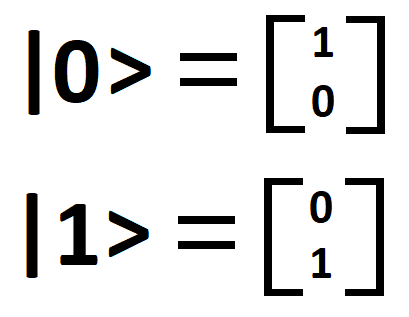
We call the two states above (|0> and |1>) the basis states from which all other states are measured. Quantum states and states, in general, are therefore defined by a string of basis states specifying the possible evolutions of those composed states.
Qubits can be reasoned about in at least three ways:
1. The Bloch Sphere
Each qubit can be represented as a specific position on the surface of a sphere having a radius of 1 (thinking in radians). Technically, the surface of that sphere is a Complex Hilbert Space! Indeed, the representation of a qubit in this way follows as a result of the underlying complex numbers at play.
Here's a fantastic graphical representation that illuminates this a bit better:
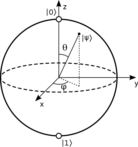
Source: WikiMedia Commons.
See how |0> and |1> are located at the poles?
A helpful rule of thumb: No other state (e.g. |1111> or |1001>) will be located at the poles of a Bloch sphere - only our basis states!
2. Ket or Dirac Notation
As we have seen, qubits unlike classical bits can be easily represented as positions on the surface of a sphere having a radius of 1 (radians-wise).
So we have seen how a qubit can, therefore, be represented by a sequence of 1's and 0's specifying a location on the surface of that sphere.
We thus arrive at ket (vector) notation which captures this intuitive notion:
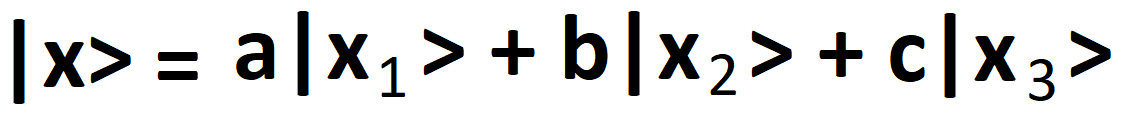
Here, |x> is called the quantum state and represents a linear combination of probability amplitudes and their respective states in superposition.
So, given |ψ> = a|0> + b|1> it follows that |a|^2 + |b|^2 = 1 where, a and b represent the probability amplitudes of their respective states.
Ket or Dirac Notation is the most common way of representing both quantum states and qubits.
3. Via (column) Vectors
We can happily translate our ket notation into (column) vector notion like so:
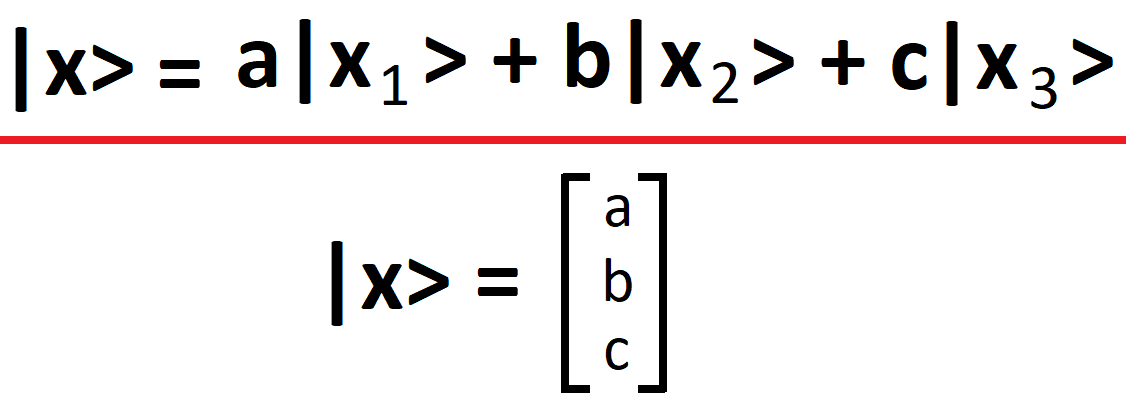
Whereby each element in the column vector represents a probability amplitude of a respective state. Such notation is useful when performing linear operations via Quantum Gates.
We easily see that operations on qubits are performed using a mix of Matrix Multiplication, Complex Numbers, and Quantum Logic Operators rather than the simple truth-functional operators of Boolean Algebra:
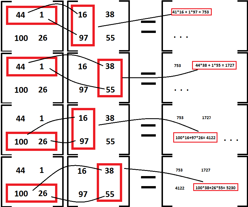
(Matrix Multiplication)
The best quantum computers that are presently publically available can handle about 20 qubits at a time, and the most powerful quantum computers top off at around 50 simultaneously.
Linear Operators (Operations on Qubits)
Quantum Logic Gates are fundamentally distinct from their Classical Logic Gate brethren, and we can see just how much so by exploring the most fundamental logical operation and its equivalent in both kinds of computational systems.
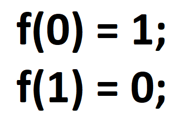
A Boolean NOT operation is a simple truth-function that negates or "reverses" the supplied inputted truth value (a 0 returns a 1 and a 1 returns a 0):
Quantum NOT (the Pauli-X linear operator below) transforms one basis state into its corresponding, "opposite", pair (|0> returns a |1> and |1> and |0>) using matrix multiplication tables:
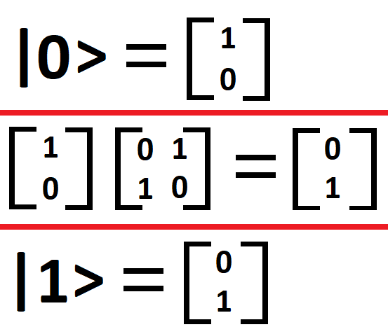
Thus, while the Quantum NOT operator (the Pauli-X linear operator) bears a superficial resemblance to the Boolean NOT operator, those superficial distinctions are immediately dispelled upon close inspection - we readily see how much more is going on with Quantum Computation for something as simple as even the most fundamental logical operation.
Unitary Evolution
It's common knowledge that observation of the wave-function results in a single observed outcome for a quantum state in superposition. Whether that's the product of observation (measurement) itself, wave-function collapse, or branching world-lines (à la Many Worlds Interpretation or Bohmian Mechanics) is still hotly debated in the Foundations of Physics and the Philosophy of Science.
For our intents and purposes, it suffices to note that measurement of a quantum state in superposition results in a resultant outcome (setting aside the fun and interesting philosophical quibbles).
Unitary Evolution, on the other hand, represents manipulation of the underlying quantum system prior to measurement rather than the measurement or collapse of the wave-function to a specific observed state. Essentially, Unitary Evolution allows us to transform an entangled quantum system in superposition prior to generating a final value.
Quantum Programming
Now that we have an idea of what's going on under-the-hood, let's take a look at two great Quantum Programming implementations: one in Python - the qiskit-sdk used in IBM's quantum cloud and one in JavaScript - jsqubits so we cover two of the most popular programming languages!
QISKit-SDK
The new qiskit-sdk provided by IBM in Python allows for local and true cloud Quantum Computing (using IBM's shiny new Quantum Computer available to all)!We'll also use Python 3.6 to get us going!
Per the official docs, there are four parts to running a QISKit program:
1. Declaring registers and configuration
In this stage, we declare how many qubits and classical bits we'll be handling:
    q = QuantumRegister(2)
    c = ClassicalRegister(2)
    qc = QuantumCircuit(q, c)
2. Putting the system into superposition
Then we can apply linear operations on our selected qubits:
qc.y(q[0])
3. Measuring the system
We can perform measurements on the quantum system returning and allowing access to a resultant state throughout:
qc.measure(q, c)
4. Running the program
A choice of backends is available to execute our program. We can run the program in the cloud or locally:
    job_sim = execute(qc, "local_qasm_simulator")
    sim_result = job_sim.result()
Basic Operations
Let's apply our quantum knowledge to Python!
A simple Pauli-X operation can be implemented like so:
from qiskit import QISKitError, execute
from qiskit import QuantumCircuit, ClassicalRegister, QuantumRegister

if __name__ == '__main__':
    try:
        # Prepare program
        q = QuantumRegister(2)
        c = ClassicalRegister(2)
        qc = QuantumCircuit(q, c)

        # Put qubit in superposition
        qc.x(q[0])

        # Measure quantum state
        qc.measure(q, c)

        # Execute program
        job_sim = execute(qc, "local_qasm_simulator")
        sim_result = job_sim.result()
        print("simulation: ", sim_result)
        print(sim_result.get_counts(qc))

    except QISKitError as ex:
        print('Quantum fluctuations! Eh Gad!'.format(ex))
Let's do the same for Hadamard:
from qiskit import QISKitError, execute
from qiskit import QuantumCircuit, ClassicalRegister, QuantumRegister

if __name__ == '__main__':

    try:

        # Prepare program
        q = QuantumRegister(2)
        c = ClassicalRegister(2)
        qc = QuantumCircuit(q, c)

        # Put qubit in superposition
        qc.h(q[0])

        # Measure quantum state
        qc.measure(q, c)

        # Execute program
        job_sim = execute(qc, "local_qasm_simulator")
        sim_result = job_sim.result()
        print("simulation: ", sim_result)
        print(sim_result.get_counts(qc))

    except QISKitError as ex:
        print('Quantum fluctuations! Eh Gad!'.format(ex)
Now let's collapse a wave-function or two, shall we:
Oh yeah!
jsqubits
jsqubits is another great library for learning how to program quantum-ly!
In this example, we'll combine some of the most basic operations along with Angular 5 to build a lightweight quantum application!

Basic Operations
We'll divide our NG5 app into two views, one for each set of basic operations.

Our injectable QuantumService will start with the three Pauli linear operators:
import {Injectable} from '@angular/core'
import {jsqubits} from 'jsqubits'

@Injectable()
export class QuantumService {

    private QUBIT_ZERO = '|00>';
    private QUBIT_ONE = '|01>';
    private QUBIT_COMPLEX_ONE = '(i)|01>';
    private QUBIT_MINUS_ONE = '-|01>';

    constructor() {}

    pauliX() {
        let x = jsqubits(this.QUBIT_ONE).x(0);
        return {
            initial: this.QUBIT_ONE,
            compute: x.toString(),
            expected: this.QUBIT_ZERO
        }
    }

    pauliY() {
        let y = jsqubits(this.QUBIT_ZERO).y(0);
        return {
            initial: this.QUBIT_ONE,
            compute: y.toString(),
            expected: this.QUBIT_COMPLEX_ONE
    }
    }

    pauliZ() {
        let z = jsqubits(this.QUBIT_ONE).z(0);
        return {
            initial: this.QUBIT_ONE,
            compute: z.toString(),
            expected: this.QUBIT_MINUS_ONE
        }
    }
}
We can then inject those helpers directly into our PauliComponent:
import {Component, OnInit} from "@angular/core";
import {QuantumService} from '../../services/quantum.service'

@Component({
  //...
})

export class PauliComponent implements OnInit {
    public pauliX;
    public pauliY;
    public pauliZ;
    constructor(private _quantumService: QuantumService) {  }
    ngOnInit() { this.quantumGo(); }
    quantumGo() {
        this.pauliX = this._quantumService.pauliX();
        this.pauliY = this._quantumService.pauliY();
        this.pauliZ = this._quantumService.pauliZ();
        console.log('Pauli linear operator tests done!');
    }
}

Let's enrich our QuantumService with two other basic operations - the Hadamard operator and a simple Fourier Transformation method:
import {Injectable} from '@angular/core'
import {jsqubits} from 'jsqubits'

@Injectable()
export class QuantumService {

    private QUBIT_ZERO = '|00>';
    private QUBIT_ONE_ZERO_ZERO = '|100>';
    private HADAMARD_RESULT = '(0.7071)|00> + (0.7071)|01>';
    private QFT_RESULT = '(0.5)|000> + (-0.5)|010> + (0.5)|100> + (-0.5)|110>';

    constructor() { }

    hadamard() {
        let h = jsqubits(this.QUBIT_ZERO).hadamard(0);
        return {
           initial: this.QUBIT_ZERO,
           compute: h.toString(),
           expected: this.HADAMARD_RESULT
        }
    }

    fourier() {
        let f = jsqubits(this.QUBIT_ONE_ZERO_ZERO).qft([1,2]);
        return {
            initial: this.QUBIT_ONE_ZERO_ZERO,
            compute: f.toString(),
            expected: this.QFT_RESULT
        }
    }
}
Like before, we can easily inject our new QuantumService helpers right into our HadamardComponent:
import {Component, OnInit} from "@angular/core"
import {QuantumService} from "../../services/quantum.service";

@Component({
    //...
})

export class HadamardComponent implements OnInit {
    public hadamard;
    public fourier;
    constructor(private _quantumService: QuantumService) {  }
    ngOnInit() { this.quantumGo(); }
    quantumGo() {
        this.hadamard = this._quantumService.hadamard();
        console.log('Hadamard test done!');
        this.fourier = this._quantumService.fourier();
        console.log('Fourier transform test done!');
    }
}
Conclusion
That concludes our quick look at Quantum Computation and the great libraries qiskit-sdk used in IBM's quantum cloud and the great JavaScript library jsqubits!
All the qubits and code used in this article can be clone from GitHub here!
Until next time!
Shout Outs!
Thanks to these great photographers for their outstanding work:
For more quantum math check out:


